Overview
"If you can't explain it simply, you don't understand it well enough."
Albert EinsteinIntroduction to Kalman Filter
The Kalman Filter is a powerful algorithm for estimating and predicting system states in the presence of uncertainty. It is a fundamental tool in fields such as target tracking, navigation, and control.
Although the Kalman Filter is a straightforward concept, many resources introduce the Kalman Filter in a way that demands an extensive mathematical background and often lack practical examples or illustrations. This makes the subject appear more complicated than it really is.
This tutorial takes a different approach. It is based on numerical examples and intuitive explanations, making the Kalman Filter accessible and easy to understand. By the end, you will not only grasp the concept and the mathematics behind it but also be able to design and apply the Kalman Filter yourself.
Problem Statement
We begin by formulating the problem to understand why we need an algorithm for state estimation and prediction.
To illustrate this, consider the example of a tracking radar:
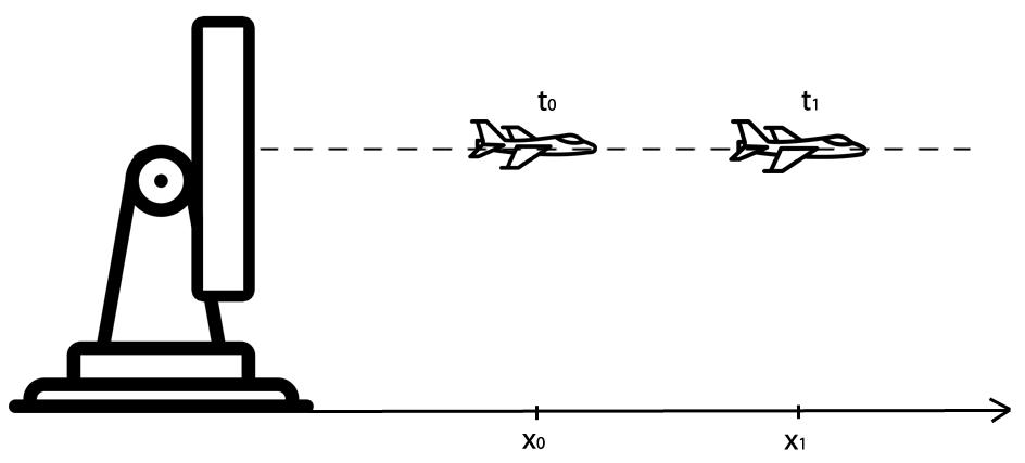
Suppose we have a radar that tracks an airplane. In this scenario, the airplane is the system, and the quantity we want to estimate is the airplane's position, which represents the system state.
The radar samples the target by steering a narrow pencil beam toward it and provides position measurements of the airplane. Based on these measurements, we can estimate the system state (the airplane position).
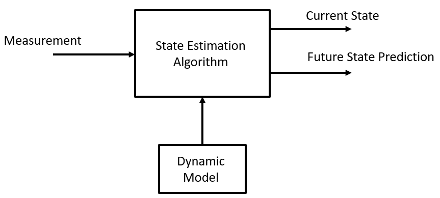
To track the airplane, the radar must revisit the target at regular intervals by pointing the pencil beam in its direction. This means the radar must be able to predict the airplane's future position for the next beam. If it fails to do so, the beam may be pointed in the wrong direction, resulting in a loss of track. To make this prediction, we need some knowledge about how the airplane moves. In other words, we need a model that describes the system's behavior over time, known as the dynamic model.
To simplify the example, let us consider a one-dimensional world, where the airplane moves along a straight line either toward the radar or away from it.

The system state is defined as the range of the airplane from the radar, denoted by \( x \). The radar sends a pulse toward the airplane, which reflects off the target and returns to the radar. By measuring the time elapsed between the transmission and reception of the pulse and knowing that the pulse is an electromagnetic wave traveling at the speed of light, the radar can easily calculate the airplane's range \( x \). In addition to range, the radar can also measure the airplane's velocity \( v \), just like a police radar gun detects a car’s speed by using the Doppler effect.
Let us assume that at time \( t_{0} \), the radar measures the airplane's range and velocity with very high accuracy and precision. The measured range is 10,000 meters, and the velocity is 200 meters per second. This gives us the system state:
\[ x_{t_{0}} = 10,000m \]
The next step is to predict the system state at time \( t_{1}=t_{0}+\Delta t \), where \( \Delta t \) is the target revisit time. Given that the airplane is expected to maintain a constant velocity, a constant velocity dynamic model can be used to predict its future position.
The distance traveled during the time interval \( \Delta t \) is given by:
\[ \Delta x = v \cdot \Delta t \]
Assuming a sampling interval of 5 seconds, the predicted position at time \( t_{1} \) is:
\[ x_{t_{1}} = x_{t_{0}} + \Delta x = 10,000 + 200 \cdot 5 = 11,000m \]
This is an elementary algorithm built on simple principles. The current system state is derived from the measurement, and the dynamic model is used to predict the future state.

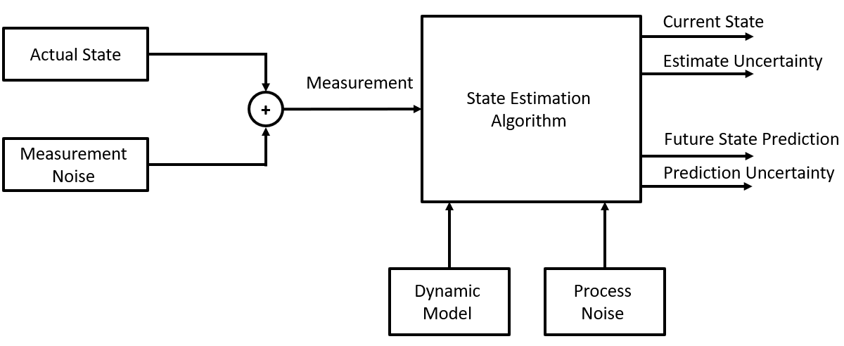
In real life, things are more complex. First, the radar measurements are not perfectly precise. It is affected by noise and contains a certain level of randomness. If ten different radars were to measure the airplane’s range at the same moment, they would produce ten slightly different results. These results would likely be close to each other, but not identical. The variation in measurements is caused by measurement noise.
This leads to a new question: How certain is our estimate? We need an algorithm that not only provides an estimate but also tells us how reliable that estimate is.
Another issue is the accuracy of the dynamic model. While we may assume that the airplane moves at a constant velocity, external factors such as wind can introduce deviations from this assumption. These unpredictable influences are referred to as process noise.
Just as we want to assess the certainty of our measurement-based estimate, we also want to understand the level of confidence in our prediction.
The Kalman Filter is a state estimation algorithm that provides both an estimate of the current state and a prediction of the future state, along with a measure of their uncertainty. Moreover, it is an optimal algorithm that minimizes state estimation uncertainty. That is why the Kalman Filter has become such a widely used and trusted algorithm.

About this tutorial
Before exploring the Kalman Filter, let me briefly introduce this tutorial.
Back in 2017, I created an online tutorial based on numerical examples and intuitive explanations to make the topic more accessible and understandable. The online tutorial provides introductory material covering the univariate (one-dimensional) and multivariate (multidimensional) Kalman Filters.
Over time, I have received many requests to include more advanced topics, such as non-linear Kalman Filters (Extended Kalman Filter and Unscented Kalman Filter), sensors fusion, and practical implementation guidelines.
Based on the material covered in the online tutorial, I authored a book.
The original online tutorial is available for free access. The e-book and the source code (Python and MATLAB) for the numerical examples are available for purchase.
The book takes the reader from the basics to the advanced topics, covering both theoretical concepts and practical applications. The writing style is intuitive, prioritizing clarity of ideas over mathematical rigor, and it approaches the topic from a philosophical perspective before delving into quantification.
The book contains many illustrative examples, including 14 fully solved numerical examples with performance plots and tables. Examples progress in a paced, logical manner and build upon each other.
The book also includes the necessary mathematical background, providing a solid foundation to expand your knowledge and help to overcome your math fears.
Upon finishing this book, you will be able to design, simulate, and evaluate the performance of the Kalman Filter.
The book includes four parts:
-
Part 1 serves as an introduction to the Kalman Filter, using eight numerical examples, and doesn't require any prior mathematical knowledge. You can call it "The Kalman Filter for Dummies," as it aims to provide an intuitive understanding and develop "Kalman Filter intuition." Upon completing Part 1, readers will thoroughly understand the Kalman Filter's concept and be able to design a univariate (one-dimensional) Kalman Filter.
Most of this part is available for free access!
-
Part 2 presents the Kalman Filter in matrix notation, covering the multivariate (multidimensional) Kalman Filter. It includes a mathematical derivation of Kalman Filter equations, dynamic systems modeling, and two numerical examples. This section is more advanced and requires basic knowledge of Linear Algebra (only matrix operations). Upon completion, readers will understand the math behind the Kalman Filter and be able to design a multivariate Kalman Filter.
Most of this part is available for free access!
- Part 3 is dedicated to the non-linear Kalman Filter, which is essential for mastering the Kalman Filter since most real-life systems are non-linear. This part begins with a problem statement and describes the differences between linear and non-linear systems. It includes derivation and examples of the most common non-linear filters: the Extended Kalman Filter and the Unscented Kalman Filter.
- Part 4 contains practical guidelines for Kalman Filter implementation, including sensor fusion, variable measurement uncertainty, treatment of missing measurements, treatment of outliers, and the Kalman Filter design process.
"The road to learning by precept is long, by example short and effective."
Lucius SenecaAbout the author
My name is Alex Becker, and I am a radar engineer with over 20 years of experience in wireless technologies, specializing in system engineering, signal processing, and Kalman Filters for tracking applications. Throughout my career, I’ve honed the skill of explaining complex topics in a simple way, making advanced concepts easier to grasp.
Constructive criticism is always welcome. I would greatly appreciate your comments and suggestions. The book's third edition has been enriched based on your insights, offering more comprehensive explanations for challenging topics. Please don't hesitate to email me with your thoughts.

About the Kalman Filter
Many modern systems utilize multiple sensors to estimate hidden (unknown) states through a series of measurements. For instance, a GPS receiver can estimate location and velocity, where location and velocity represent the hidden states, while the differential time of the arrival of signals from satellites serves as measurements.
One of the biggest challenges of tracking and control systems is providing an accurate and precise estimation of the hidden states in the presence of uncertainty. For example, GPS receivers are subject to measurement uncertainties influenced by external factors, such as thermal noise, atmospheric effects, slight changes in satellite positions, receiver clock precision, and more.
The Kalman Filter is a widely used estimation algorithm that plays a critical role in many fields. It is designed to estimate the hidden states of the system, even when the measurements are imprecise and uncertain. Also, the Kalman Filter predicts the future system state based on past estimations.
The filter is named after Rudolf E. Kálmán (May 19, 1930 – July 2, 2016). In 1960, Kálmán published his famous paper describing a recursive solution to the discrete-data linear filtering problem.

