Overview

"If you can't explain it simply, you don't understand it well enough."

Albert Einstein

About this tutorial

The Kalman Filter algorithm is a powerful tool for estimating and predicting system states in the presence of uncertainty and is widely used as a fundamental component in applications such as target tracking, navigation, and control.

Although the Kalman Filter is a straightforward concept, many resources on the subject require extensive mathematical background and fail to provide practical examples and illustrations, making it more complicated than necessary.

Back in 2017, I created an online tutorial based on numerical examples and intuitive explanations to make the topic more accessible and understandable. The online tutorial provides introductory material covering the univariate (one-dimensional) and multivariate (multidimensional) Kalman Filters.

Over time, I have received many requests to include more advanced topics, such as non-linear Kalman Filters (Extended Kalman Filter and Unscented Kalman Filter), sensors fusion, and practical implementation guidelines.

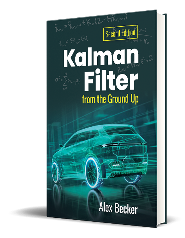
Based on the material covered in the online tutorial, I authored a book.

The original online tutorial is available for free access. The e-book and the source code (Python and MATLAB) for the numerical examples are available for purchase.

The book takes the reader from the basics to the advanced topics, covering both theoretical concepts and practical applications. The writing style is intuitive, prioritizing clarity of ideas over mathematical rigor, and it approaches the topic from a philosophical perspective before delving into quantification.

The book contains many illustrative examples, including 14 fully solved numerical examples with performance plots and tables. Examples progress in a paced, logical manner and build upon each other.

The book also includes the necessary mathematical background, providing a solid foundation to expand your knowledge and help to overcome your math fears.

Upon finishing this book, you will be able to design, simulate, and evaluate the performance of the Kalman Filter.

The book includes four parts:

Part 1 serves as an introduction to the Kalman Filter, using eight numerical examples, and doesn't require any prior mathematical knowledge. You can call it "The Kalman Filter for Dummies," as it aims to provide an intuitive understanding and develop "Kalman Filter intuition." Upon completing Part 1, readers will thoroughly understand the Kalman Filter's concept and be able to design a univariate (one-dimensional) Kalman Filter.
Most of this part is available for free access!
Part 2 presents the Kalman Filter in matrix notation, covering the multivariate (multidimensional) Kalman Filter. It includes a mathematical derivation of Kalman Filter equations, dynamic systems modeling, and two numerical examples. This section is more advanced and requires basic knowledge of Linear Algebra (only matrix operations). Upon completion, readers will understand the math behind the Kalman Filter and be able to design a multivariate Kalman Filter.
Most of this part is available for free access!
Part 3 is dedicated to the non-linear Kalman Filter, which is essential for mastering the Kalman Filter since most real-life systems are non-linear. This part begins with a problem statement and describes the differences between linear and non-linear systems. It includes derivation and examples of the most common non-linear filters: the Extended Kalman Filter and the Unscented Kalman Filter.
Part 4 contains practical guidelines for Kalman Filter implementation, including sensor fusion, variable measurement uncertainty, treatment of missing measurements, treatment of outliers, and the Kalman Filter design process.

Get the book

"The road to learning by precept is long, by example short and effective."

Lucius Seneca

About the Kalman Filter

Many modern systems utilize multiple sensors to estimate hidden (unknown) states through a series of measurements. For instance, a GPS receiver can estimate location and velocity, where location and velocity represent the hidden states, while the differential time of the arrival of signals from satellites serves as measurements.

One of the biggest challenges of tracking and control systems is providing an accurate and precise estimation of the hidden states in the presence of uncertainty. For example, GPS receivers are subject to measurement uncertainties influenced by external factors, such as thermal noise, atmospheric effects, slight changes in satellite positions, receiver clock precision, and more.

The Kalman Filter is a widely used estimation algorithm that plays a critical role in many fields. It is designed to estimate the hidden states of the system, even when the measurements are imprecise and uncertain. Also, the Kalman Filter predicts the future system state based on past estimations.

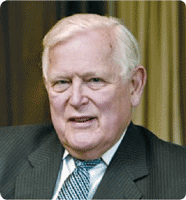
The filter is named after Rudolf E. Kálmán (May 19, 1930 – July 2, 2016). In 1960, Kálmán published his famous paper describing a recursive solution to the discrete-data linear filtering problem.

The prediction requirement

Before delving into the Kalman Filter explanation, let us first understand the necessity of a tracking and prediction algorithm.

To illustrate this point, let's take the example of a tracking radar.

Suppose we have a track cycle of 5 seconds. At intervals of 5 seconds, the radar samples the target by directing a dedicated pencil beam.

Once the radar "visits" the target, it proceeds to estimate the current position and velocity of the target. The radar also estimates (or predicts) the target's position at the time of the next track beam.

The future target position can be easily calculated using Newton's motion equations:

\[ x= x_{0} + v_{0} \Delta t+ \frac{1}{2}a \Delta t^{2} \]

Where:

\( x \)	is the target position
\( x_{0} \)	is the initial target position
\( v_{0} \)	is the initial target velocity
\( a \)	is the target acceleration
\( \Delta t \)	is the time interval (5 seconds in our example)

If you need a refresh on the motion equations, refer to Appendix I in the book.

When dealing with three dimensions, Newton's motion equations can be expressed as a system of equations:

\[ \left\{\begin{matrix} x= x_{0} + v_{x0} \Delta t+ \frac{1}{2}a_{x} \Delta t^{2}\\ y= y_{0} + v_{y0} \Delta t+ \frac{1}{2}a_{y} \Delta t^{2}\\ z= z_{0} + v_{z0} \Delta t+ \frac{1}{2}a_{z} \Delta t^{2} \end{matrix}\right. \]

The set of target parameters \( \left[ x, y, z, v_{x},v_{y},v_{z},a_{x},a_{y},a_{z} \right] \) is known as the System State. The current state serves as the input for the prediction algorithm, while the algorithm's output is the future state, which includes the target parameters for the subsequent time interval.

The system of equations mentioned above is known as a Dynamic Model or State Space Model. The dynamic model describes the relationship between the input and output of the system.

Apparently, if the target's current state and dynamic model are known, predicting the target's subsequent state can be easily accomplished.

In reality, the radar measurement is not entirely accurate. It contains random errors or uncertainties that can affect the accuracy of the predicted target state. The magnitude of the errors depends on various factors, such as radar calibration, beam width, and signal-to-noise ratio of the returned echo. The random errors or uncertainties in the radar measurement are known as Measurement Noise.

In addition, the target motion is not always aligned with the motion equations due to external factors like wind, air turbulence, and pilot maneuvers. This misalignment between the motion equations and the actual target motion results in an error or uncertainty in the dynamic model, which is called Process Noise.

Due to the Measurement Noise and the Process Noise, the estimated target position can be far away from the actual target position. In this case, the radar might send the track beam in the wrong direction and miss the target.

In order to improve the radar's tracking accuracy, it is essential to employ a prediction algorithm that accounts for both process and measurement uncertainty.

The most common tracking and prediction algorithm is the Kalman Filter.

Get the book